MATSIRO (Takata et al., 2003) is the land surface scheme of an Atmospheric Ocean General Circulation Model, the Model for Interdisciplinary Research On Climate (MIROC; Hasumi et al., 2004 ; Watanabe et al., 2010 ), jointly developed by the Atmosphere and Ocean Research Institute at the University of Tokyo, the National Institute of Environmental Studies, and the Frontier Research Center for Global Change in Japan.
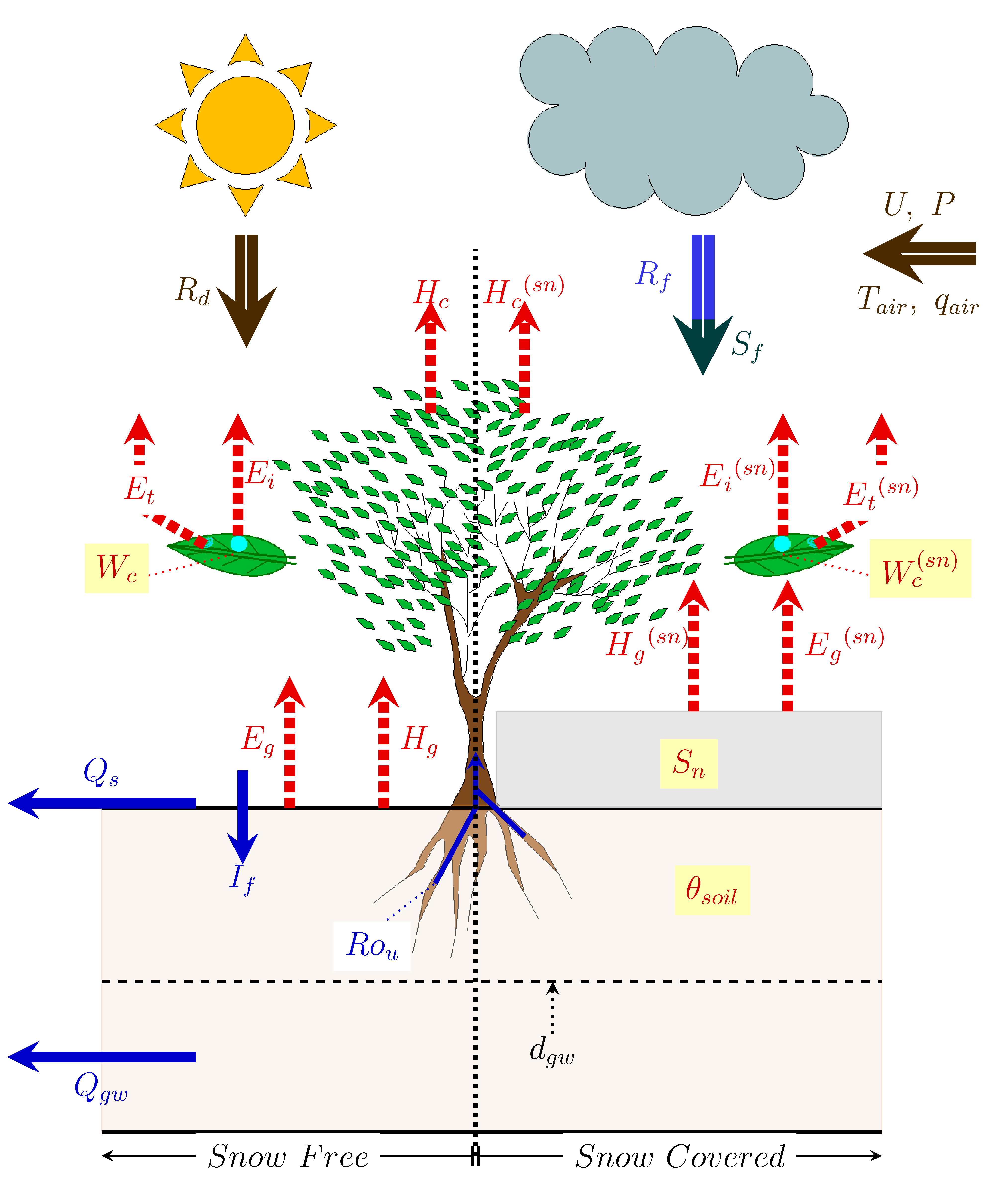 Fig. 1: Schematic diagram of the MATSIRO LSM |
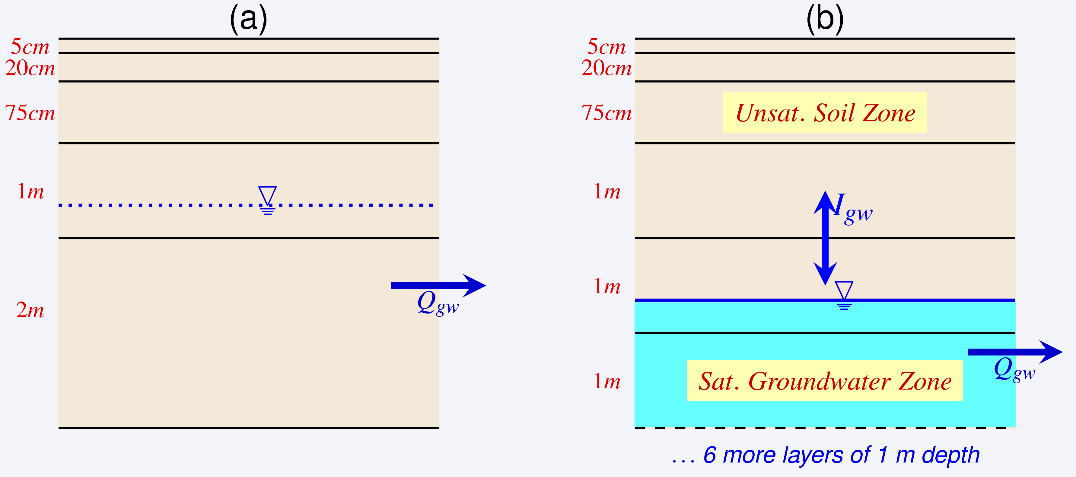 Fig. 2: Schematic representation of soil layers and their resolution in (a) MATSIRO and (b) MATSIRO with groundwater |
A schematic representation of the original MATSIRO is presented in Figure 1. Energy fluxes are calculated at both ground and canopy surfaces in the snow-free and snow-covered fractions of a grid cell considering subgrid snow distribution. Interception loss from the canopy and transpiration are estimated on the basis of photosynthesis scheme of SiB2 [Sellers et al., 1986, 1996].
Soil column is divided into five layers (Figure 2a) and the temperature and moisture (liquid and frozen) are calculated for each layer. The thickness of soil layers is 5, 20, 75, 100 and 200 cm respectively from ground surface. The WTD is implicitly estimated from the unsaturated matric potential of the lowermost soil layer as,
![]()
where dgw is WTD (always <4 m), Zg is the depth to the lowermost soil layer, and ψkWT is the unsaturated matric potential of the lowermost soil layer. The Richards’ equation [Richards, 1931] is solved for all soil layers irrespective of the location of water table as there is no explicit representation of saturated zone.
A simplified version of TOPMODEL [Beven and Kirkby, 1979] developed by Stieglitz et al. (1997) is adopted to represent runoff process. Baseflow is calculated as,
![]()
where K0[L T−1] is the saturated hydraulic conductivity at ground surface, fatn[−] is the attenuation coefficient of K0 with depth, tanβs[−] is the mean topographic slope within a grid cell, and Ls is the length of a conceptual hillslope which is inversely proportional to tanβs.
Although the majority of hydrologic processes are physically represented in MATSIRO, it lacks a proper representation of groundwater processes. A simple, lumped unconfined aquifer model (Yeh and Eltahir, 2005a, b) is integrated into MATSIRO. One-dimensional lumped water balance equation for the unconfined aquifer can be expressed as,
![]()
where Sy[-] is the specific yield, dgw is the WTD, Igw[L T−1] is GW recharge to (when positive) or capillary rise from (when negative) the GW reservoir, and Qgw[L T−1] is the baseflow.
The difference between recharge and baseflow determines the fluctuations of water table. The reservoir is nonlinear because both Igw and Qgw have complex nonlinear dependencies on dgw. The Igw depends on the degree of saturation of the lowermost soil layer. The GW reservoir is dynamic in that the exact location of the water table determines the number of soil layers in unsaturated zone, for which the soil moisture-based Richards’ equation is solved.
In order to accommodate the variable WTD and accurately locate its position, soil column is extended to 10 m below the ground surface -in total 12 layers with the depth of 5, 20, and 75 cm for the top 3 layers, and 1 m each for the remaining 9 layers. A schematic representation of the linkage of the soil-groundwater model in MATSIRO-Groundwater Model is presented in Figure 2b. Unlike original MATSIRO, the soil column now has an explicit representation of unsaturated and saturated zones separated by the water table.
The TOPMODEL-based baseflow is replaced by the following threshold relationship developed based on observations in Illinois by Yeh and Eltahir (2005a)

where K [T−1] is the outflow constant, and d0 is the threshold WTD shallower than which baseflow is initialized. Both d0 and dgw are taken as positive values. Yeh and Eltahir (2005b) accounted for the subgrid heterogeneity of WTD by using a statistical-dynamical approach based on the spatial distribution of the observed WTD in Illinois. The derived grid-scale (macroscale) average baseflow can be written as [Yeh and Eltahir,2005b, equation (5)]

where Γ (α) is the Gamma function, and α and λ are the shape and scale parameters, respectively, of the assumed Gamma distribution of dgw. The d0, K and Sy are the main GW parameters.
References:
Beven, K. J. and M. J. Kirkby, 1979: A physically based variable contributing area model of basin hydrology. Hydrol. Sci. Bull., 24, 43–69, doi:10.1080/02626667909491834.
Hasumi, H., S. Emori, A.-O. A., and co authors, 2004: K-1 coupled GCM (MIROC) description. Tech. Rep. 1, Center for Climate System Research (CCSR), University of Tokyo and National Institute of Environmental Studies (NIES) and Frontier Research Center for Global Change (FRCGC).
Richards, L. A., 1931: Capillary conduction of liquids through porous mediums. Physics, 1 (5), 318–333, doi:10.1063/1.1745010.
Sellers, P. J., Y. Mintz, Y. C. Sud, and A. Dalcher, 1986: A simple biosphere model (SiB) for use with general circulation models. J. Atmos. Sci., 43, 505–531, doi:10.1175/1520-0469(1986)043<0505:ASBMFU>2.0.CO;2.
Sellers, P. J., D. A. Randall, C. J. Collatz, J. A. Berry, C. B. Field, and D. A. Dazlich, 1996: A revised land surface parameterization (SiB2) for atmo¬spheric GCMs. Part 1: Model formulation. J. Clim., 9, 676–705, doi:10.1175/1520¬0442(1996)009<0676:ARLSPF>2.0.CO;2.
Stieglitz, M., D. Rind, J. S. Famiglietti, and C. Rosenzweig, 1997: An efficient approach to modeling the topographic control of surface hydrology for re¬gional and global climate modeling. J. Clim., 10 (1), 118–137, doi:10.1175/1520¬0442(1997)010<0118:AEATMT>2.0.CO;2.
Takata, K., S. Emori, and T. Watanabe, 2003: Development of minimal advanced treatments of surface interaction and runoff. Global Planet. Change, 38, 209–222, doi: 10.1016/S0921-8181(03)00030-4.
Watanabe, M., et al., 2010: Improved climate simulation by MIROC5: Mean states, variability, and climate sensitivity. J. Clim., 23 (23), 6312–6335, doi: 10.1175/2010JCLI3679.1.
Yeh, P. J.-F. and E. A. B. Eltahir, 2005a: Representation of water table dynamics in a land surface scheme. Part I: Model development. J. Clim., 18, 1861–1880, doi: 10.1175/JCLI3330.1.
Yeh, P. J.-F. and E. A. B. Eltahir, 2005b: Representation of water table dynamics in a land surface scheme. Part II: Subgrid variability. J. Clim., 18, 1881–1901, doi: 10.1175/JCLI3331.1.