Rhône AGG Description/Documentation

    The Rhône is the largest European river which empties into the Mediterranean Sea. The corresponding basin covers a significant region of south-eastern France, encompassing a large range in climatic conditions (continental, Mediterranean and Alpine climates) and surface characteristics (bare mountains, forest, crop land, etc.). An outline of the Rhône basin model domain is shown relative to France and western Europe in Fig. 2.1. Surface characteristics, sub-surface parameters and atmospheric forcing have been mapped onto this domain for use in atmospheric and hydrological model studies. The atmospheric forcing, the surface vegetation and soil parameter database, and the river discharge and snow depth observation data are described in detail in Habets et al. (1999b), Etchevers et al. (2001), Golaz et al. (2001) and Ottlé et al. (2001).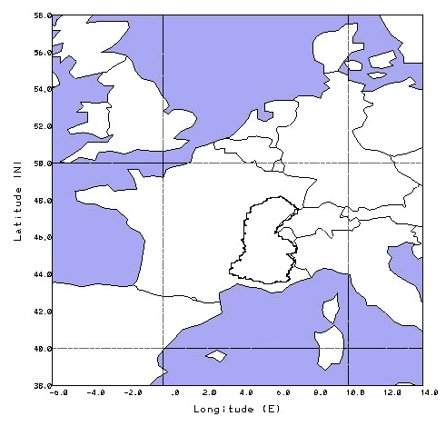

FIG. 2.1 The Rhône basin model domain (highlighted area).

Atmospheric Forcing

    The domain is divided up into 1471 8 km x 8 km grid boxes for the atmospheric forcing (Fig. 2.2). The forcing is calculated using the SAFRAN (Systême d'Analyse Fournissant des Reseignements Atmosphérique a la Neige) analysis system (Durand et al. 1993), which was designed to compensate for the large variation in elevation in the Rhône Alps (0-4800 m). The topography used for the 8x8 km grid is shown in Fig. 2.3. The atmospheric data utilized by the system consist of standard screen level observations at approximately 60 Météo-France weather network sites within the domain, ECMWF analysis and climatological data. In addition, total daily precipitation data from over 1500 gauges are incorporated into the system. The basin is divided into 249 homogeneous climatic zones which have a unique set of climatological parameters. The locations of the climatic zones (outlined), rain gauges (crosses) and meteorological stations (filled triangles) are shown in Fig. 2.4.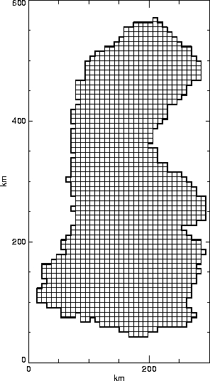

FIG. 2.2 The meteorological grid used for the SVAT scheme. There are 1471 8 km x 8 km grid boxes within the Rhône domain.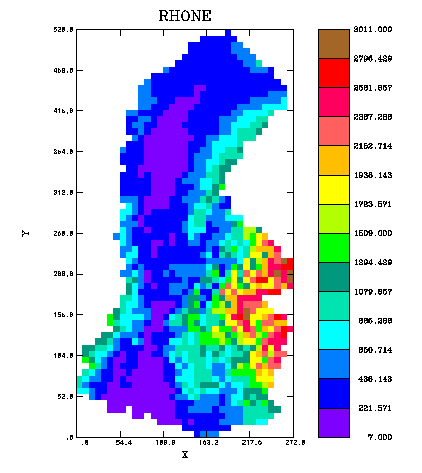

FIG. 2.3 The 8x8 km topography for the Rhône basin model domain.

    SAFRAN computes the vertical profile of each of the atmospheric variables every six hours within each climatic zone. The parameters are then interpolated to one hour intervals and to the grid. The total daily precipitation is analyzed using the observational data together with a vertical gradient of precipitation (with altitude) derived from climatology. The precipitation is then distributed hourly following the daily cycle of observed humidity and the weather type (again from climatology). Precipitation is partitioned between rainfall and snowfall based on the 0.5 C isotherm (see Habets et al. 1999b for more details).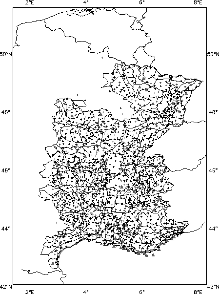

FIG. 2.4 The locations of the climatic zones (outlined), daily rain gauges (crosses) and meteorological stations (red triangles) used by SAFRAN to derive the atmospheric forcing.

    Downwelling radiative fluxes are calculated using the radiative transfer scheme of Ritter and Geleyn (1992) together with ECMWF and cloudiness analyses. The forcing extracted from SAFRAN for the Soil Vegetation Atmosphere Transfer (SVAT) model computational grid is available at a three hour time step. The provided forcing variables are; air temperature at 2 m (T_a: K), wind speed at 10 m (V_a: m s^-1), specific humidity at 2 m (q_a: kg kg^-1), down-welling visible solar radiation (R_g: W m^-2), down-welling long-wave atmospheric radiation (R_at: W m^-2), liquid precipitation rate (P_l: kg m^-2 s^-1) and liquid water equivalent snow/solid precipitation rate (P_s: kg m^-2 s^-1). The surface pressure (p: Pa) only varies as a function of altitude, but the input values are provided at the same time step as the other forcings (for ease of usage by the models). Problems relating to model partitioning of precipitation into snow and rain are avoided as the distinct components are provided. The forcing variable definitions, sign conventions and units follow the ALMA land-surface data convention.

    Forcing is available for 17 years (1981-1998), however, only four years will be used in the current study (August 1, 1985-July 31, 1989). These particular years were selected in order to be consistent with the GSWP (Dirmeyer et al. 1999) database. The starting and ending times are during the summertime due to the importance of a good initialization of the snow cover in the mountainous regions.

    The 4-year average liquid and solid precipitation components are shown in Fig. 2.5, and the 5 other 4-year average forcing variables (together with the total precipitation) at each grid point are shown in Fig. 2.6. The monthly domain-average forcing variables for the period August 1, 1985, through July 31, 1989, are shown in Fig 2.7. The winter seasons in 1985-1986 and 1986-1987 were two of the three coldest in the forcing dataset for the period 1981-1998 (the other exceptionally cold winter was in 1984-1985).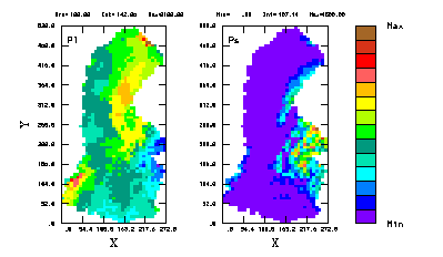

FIG 2.5 The 4-year average precipitation forcing variables from the Rhône database from August 1, 1985 to July 31, 1989: P_l (liquid: 100-2100 with an interval of 143) and P_s (solid: 0-1500 with an interval of 107) in kg m^-2.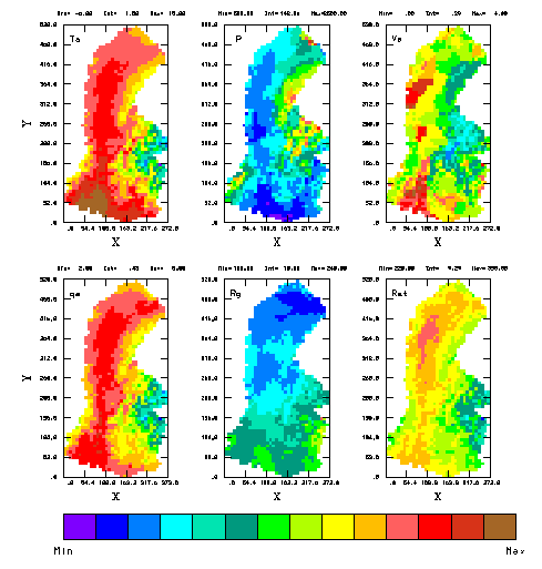

FIG 2.6 The 4-year average forcing variables from the Rhône database from August 1, 1985 to July 31, 1989: T_a (C: -6 - 15 with an interval of 1.5), P (kg m^-2: 500-2500 with an interval of 143), V_a (m s^-1: 0-4 with an interval of 0.29), q_a (g kg^-1: 2-8 with an interval of 0.43), R_g (W m^-2: 100-240 with an interval of 10) and R_at (W m^-2: 220-350 with an interval of 9.3).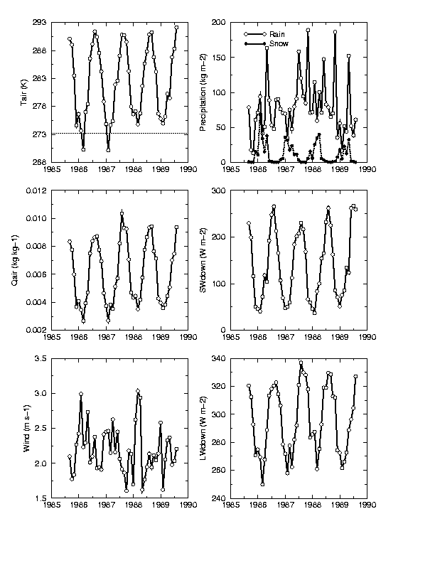

FIG 2.7 The 4-year domain-average monthly mean forcing variables from the Rhône database from August 1, 1985 to July 31, 1989.

Soil and Vegetation Parameters

    Soil and vegetation parameter data are available at the same spatial resolution as the atmospheric forcing. The soil parameters are defined using the soil textural properties (sand and clay fractions) from the INRA soil database (King et al. 1995). The spatial distributions of the sand and clay fractions are shown in Fig.s 2.8a and 2.8b, respectively.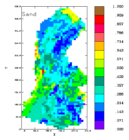

FIG. 2.8 The soil sand fraction for each grid box.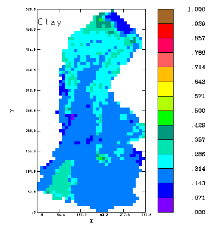

FIG. 2.8 The soil clay fraction for each grid box.

    The vegetation parameters are defined using a vegetation map from the Corine Land cover Archive (Giordano et al. 1990) and a two-year satellite archive of the AVHRR/NDVI Index (Champeaux and Legléau, 1995). There are 10 distinct surface types considered, and the relative fractional coverage of each surface type within each grid box was used to determine average values for the 8 km x 8 km grid boxes. The 10 dominant surface types are listed with their corresponding index in Table 2.1. The dominant surfaces are shown in Fig. 2.9; bare rock (9), deciduous forest (10), coniferous forest (8), grassland (7), cereal crops (3 and 5), crops other than cereals (1, 2 and 4), and mixed grassland and crops (6).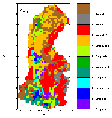

FIG 2.9 The dominant land classification for each grid cell; 1) crops type A, 2) Mediterranean crops, 3) cereals type A, 4) crops type B, 5) cereals type B, 6) crops and grassland, 7) grassland, 8) coniferous forest, 9) rocks/bare soil and 10) deciduous forest.

    Maximum and minimum vegetation parameter values are determined for each class. These values are then used with the monthly observed NDVI to determine the evolution of the roughness length, vegetation cover fraction and Leaf Area Index (LAI). Similar surface types (such as Cereals A and B) can have different temporal evolutions due to differences in the observed NDVI. The single annual cycle for these parameters is to be applied to all years simulated by the participant models. See Habets et al. (1999b) and Etchevers et al. (2001) for more details.

Distributed hydrological model data

    Surface and sub-surface hydrological grids have also been defined for use by distributed hydrological models. Topographical data is used to determine the surface hydrographic network and the water transfer time constant between each hydrological grid cell (Golaz 1999). The maximum transfer time for water to reach the outlet of the basin was calibrated using the MODCOU model together with the observed streamflow data.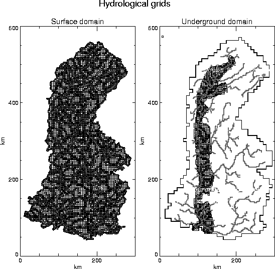

FIG 2.10 Surface and underground MODCOU grids.

    The evolution of the water table is a function of transmissivity and storage coefficients which have also been calibrated using the observed streamflow. MODCOU uses a two-layer approach, and the grid networks are shown in Fig. 2.10. The underground layer encompasses the aquifers for the Rhône and Saone valleys and is approximately 21 % of the total surface area of the basin, while the surface layer corresponds to the atmospheric forcing domain and contains 27054 grid elements.

Validation Data

    There are two sets of observations which are utilized for validating model simulations for the Rhône basin. The first consists of 24 daily snow depth observation sites located within the French Alps, which is used to evaluate the snow depth prediction and timing of Spring snow melt simulated by the snow cover module. The locations of the sites are shown in Fig. 2.11. A general evaluation will be done as the depth measurements correspond to a point or a field, and the simulated snowpack will correspond to the average value over an 8 km x 8 km grid box. The obvious drawback of using depth measurements is that model biases in simulated snow density can impact this variable. From a hydrological standpoint, the snow water equivalent (SWE) would form the basis for a more consistent inter-comparison between the models and with the observations, however, SWE was not observed. The snow depth is still useful, however, as it can be used to infer the timing of the snowpack ablation.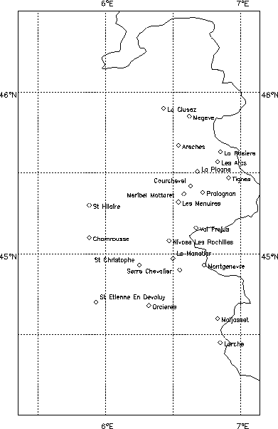

FIG. 2.11 Stations at which daily snow depth measurements are available.

    The second set of observations consist of 145 river gauges which are used for validation of the simulated streamflow. The location of the gauges for the 10 largest basins are shown in the left panel of Fig. 2.12. The relationship between the rivers and the relief is shown in the right panel. For more information, see Habets et al. (1999b) and Etchevers et al. (2001).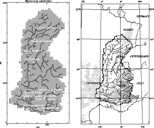

FIG. 2.12 Locations of the gauging stations for the 10 largest sub-basins within the Rhône basin are shown in the left panel. The relationship between the major rivers and the relief is shown in the right panel (from Habets et al. (1999b)).