EXP1
EXP1 of GSWP3 is a long-term retrospective experiment. It aims to investigate how interactions among energy-water- carbon cycles have changed spanning 1850-2010 using a multi-model approach over a global 0.5 deg. land grid. Since most land surface models do not have full or uniform representations of water and carbon cycles, we will include various types of models (e.g., so-called first, second and third generation land surface models, hydrologic models, ecological models, and dynamic vegetation models) and will consider time evolution of coupled processes related parameters such as land use/cover, LAI, and CO2. Also, a standard product of the project will be an extensive set of land fluxes and state variables, which has the potential to serve as a long-term land-surface reanalysis. It also will serve as a reference set for the long-term variability of various processes in the terrestrial hydro-energy-eco system that respond to surrounding large-scale climate variability, such as changes in extremes (e.g., flood and drought), land carbon balances, and water and energy inputs to the atmosphere.
Boundary Conditions
Surface meteorology
retrospective atmospheric boundary conditions (9 variables: Rainfall, Snowfall, 2m Air Temperature, 2m Specific Humidity, Surface Pressure, Downward Shortwave Radiation, Downward Longwave Radiation, 10m Wind Speed, and Cloud Cover Fraction) for 1901-2010 in 3-hourly resolution are generated. 20th Century Reanalysis (20CR) [compo2011] [Compo el al., 2011] on global 2° resolution is dynamically downscaled into T248 (~0.5°) grid using a spectral nudging technique [Yoshimura and Kanamitsu 2008] in a Global Spectral Model (GSM) [Figure 2]. This successfully keeps the low frequency signal of original reanalysis, providing additional high frequency signals, which are lacking in previous products [e.g., Weedon et al., 2011]. It is essential to investigate phenomena at higher spatiotemporal scales such as extreme events. In order to relieve known artifacts (e.g., ripple patterns and persistent overcast in high latitude region), additional techniques, such as single ensemble correction [Yoshimura and Kanamitsu, 2013] and vertically weighted damping [Hong and Chang, 2012], are applied. Model biases in the downscaled 20CR are corrected using observational data (e.g., GPCC for precipitation, SRB for short/long wave radiation, and CRU for air temperature and daily temperature range). In addition to previously introduced bias correction algorithms [e.g., Weedon et al., 2011], variability in higher temporal (<month) resolution is carefully corrected [Kim et al., in preparation]. Also, wind-induced precipitation undercatch correction is applied considering different types of gauges and their global distribution [Hirabayashi et al., 2008]. Through the above mentioned data generation strategy, GSWP3 has further reliability and consistency over the century long target timespan with higher spatiotemporal resolutions.
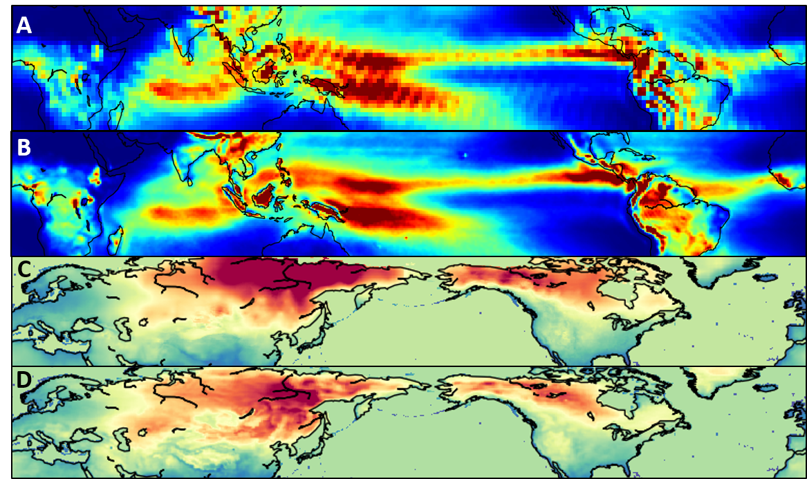
Figure 2. Comparison between Original Reanalysis (A, C) and Dynamically Downscaled Fields (B, D): Annual Surface Precipitation (A, B) and Variance of Daily 2m Temperature (C, D)
Land Use/Cover, LAI and CO2
Land cover is also treated as a time evolving variable in order to take account of anthropogenic land surface alterations. Prescribed land-use/land-cover changes are derived from the Land Use Harmonization (LUH) data set [Hurtt et al., 2006]. It is strongly recommended that the participant models incorporated with GCMs in CMIP5 use the same method to generate land use/cover maps as used in their CMIP5 experiments. Project standard maps will be provided for convenience. MODIS-based potential vegetation maps are used to generate time varying land cover grids considering human impacts. Models should use their prognostic scheme for LAI prediction when available. Climatology of LAI seasonality for each plant functional type will be prepared using the MODIS LAI product, but each modeling group can use their pre-existing parameters. Long-term variability of CO2 concentration will follow the CMIP5 protocol.
Land Sea Mask and Topography
The project standard land/sea mask and topography are derived from CRU in 0.5° global data excluding Antarctica. Spatial consistency between different dataset (e.g., observations and reanalysis) will be considered.
Soil Texture
It is recommended that modeling groups derive their own map based on soil compositions from the Harmonized World Soil Database (HWSD) [FAO/IIASA/ISRIC/ISSCAS/JRC, 2012], but it is also possible to use their existing soil texture map. As a project standard product, a HWSD-based 0.5° global map generated according to the USGS soil texture classification triangle will be provided.
Initial Conditions
Initial conditions of simulations will be prepared by each participant following the project protocol. Preceding the actual simulation period (1901-2010; section 3.2), 30-years additional forcing data (1871-1900) will be provided for model spin-up with minimal bias corrections (e.g., climatological and topographical corrections).
Model SImulations and Verification
EXP1rticipating models are categorized into three groups: no photosynthesis, static plant physiology, and dynamic plant physiology. Mandatory and optional sets of simulations for each group follow Table 1.
Verification
First order verifications of simulations (e.g., energy budget closure, water balance, carbon balance) are done by a project-provided verification interface. Extensive validation will be achieved using multiple observations for key variables by the project team. Some code snippets and a web interface will be provided for convenience.
Output Variables
The minimum set of variables to be submitted for the project is shown in Table 2. In order to bridge different modeling communities; CF and ALMA naming conventions are allowed as the standard of the GSWP3. A complete list and details will be fixed and specified on the project web page.
Data Submission
Simulation results will be submitted in compressed netCDF format (version 4). Allowing both CF and ALMA naming conventions, variable names according to the other naming convention should be given as an attribute of each variable. Output template details (e.g., dimensions and attributes) will be specified in the project web page.
| Type | Variables (up to 3houly, daily, monthly) [TENTATIVE]
|
| Energy Cycles | Net shortwave radiation, net long wave radiation, latent heat flux,
sensible heat flux, ground heat flux, change in surface heat storage,
surface temperature, change in snow cold content, …
|
| Water Cycles | Total evapotranspiration, evaporation of canopy interception,
vegetation transpiration, bare soil evaporation, open water evaporation,
ssnow sublimation, ublimation of ice from soil and canopy interception,
surface runoff, subsurface runoff, water flowing out of snowpack,
change in column soil moisture, change in soil moisture in single soil layers,
instantaneous soil moisture in single soil layers,
change in snow-water equivalent, change in surface liquid water storage,
change in canopy interception storage, potential evapotranspiration, …
|
| Carbon Cycles | Gross primary productivity, net primary productivity, net ecosystem exchanges,
autotrophic respiration, heterotrophic respiration, total respiration,
fire emissions, total living biomass, total soil carbon, …
|